Using the Crosstab Analyzer
Creating a spreadsheet in the Crosstab Analyzer:
For example, you are asked to create a Labour Costings Spreadsheet that displays the Labour Costings for all of the Victorian Cost centres of the company for the past three financial years, displayed by the months and weeks. You are also required to break this down further to show the cost per Department and identify the types of Pay Items included.
- In the Data Explorer Query Type Menu, select Labour Costing.
- Select Costing Totals in the Query Selector.
- Enter the required date range.
- Select Crosstab Analyzer as your Destination.
- Click Run Query
The Pivot Grid Field list will appear displaying all of the fields available for that specific type of query.
![]() The Data Area will not display any information at this point. It will only populate after Step 12 has been completed.
The Data Area will not display any information at this point. It will only populate after Step 12 has been completed.
- Click the Financial Year column and, holding the left mouse button down, drag it up until the green arrow indicator is positioned where it shows Drop Row Fields Here.
- Click the Departments column and, holding the left mouse button down, drag it up until the green arrow indicator is positioned to the right of the Financial Year column.
- Click the Pay Items Description column and, holding the left mouse button down, drag it up until the green arrow indicator is positioned to the right of the Departments column.
- Click the Month No column and, holding the left mouse button down, drag it up until the green arrow indicator is positioned where it shows Drop Column Fields Here.
- Click the Month column and, holding the left mouse button down, drag it up until the green arrow indicator is positioned to the right of the Month No column.
- Click the Week column and, holding the left mouse button down, drag it up until the green arrow indicator is positioned to the right of the Month column.
- Click the Amount column and, holding the left mouse button down, drag it up until the green arrow indicator is positioned where it shows Drop Data Fields Here.
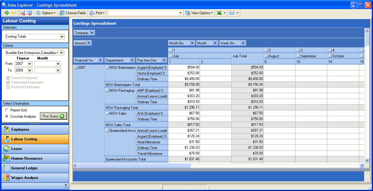
You should see the Data Area of the screen fill with your own formatted data similar to the screen shown next.
To narrow down the report's results, you can use filters. To filter your results:
- Select and drag the required filter fields onto the filter header area.
- Click on the drop-down arrow on the field header.
- From the values in the field’s drop-down list, uncheck (untick) those values that need to be filtered out.
This will affect the entire report. Values that are filtered out will not be included in the calculation totals.
![]() Field values in reports are displayed hierarchically, if two or more fields are located in the drop areas. The hierarchical view of the data allows you to analyse a report at different levels. Using the above example you can see the Financial Year and Departments columns have been dropped into the row header area. In the view you can see the way the data is summarised by the Financial Year, then by each Department
Field values in reports are displayed hierarchically, if two or more fields are located in the drop areas. The hierarchical view of the data allows you to analyse a report at different levels. Using the above example you can see the Financial Year and Departments columns have been dropped into the row header area. In the view you can see the way the data is summarised by the Financial Year, then by each Department
Once you have created and formatted a custom view, it is possible to save it for use again at a later date. To save a custom view:
- Click on the View Options button

- Select Save Current View
 from the drop-down list.
 - Enter the name you want to allocate to the new view.
- Click OK.
Once you have saved the view, it will become available in the drop down list for the current user.
Create a complex filter using 'Prefilter'
Sometimes you may have a more complex filter that you want to apply to the data. For this you may wish to use Prefilter.
![]() For further information about the features of the Crosstab Analyzer or on how to set up reports using this feature contact HR3 Support.
For further information about the features of the Crosstab Analyzer or on how to set up reports using this feature contact HR3 Support.

